Bikeshare_popular travel times
This project was completed as a part of the udacity data science with R nano degree program. The project goal was to formulate and answer some questions using the bikeshare data from three US cities.
## data.table 1.14.2 using 8 threads (see ?getDTthreads). Latest news: r-datatable.comQuestion 1: Popular times of travel
What is the most common month ? What is the most common day of week? What is the most common hour of day?
Step a) Data Cleaning and organization -
In the first R code chunk, I used data.table library to read only the columns of interest, and to create a new column ‘City’ (fill it with values Chicago, Newyork and Washington respectively) for all three data sets. I then combined all of the data tables into one using rbind. Finally, I used the stringr replace all function for replacing the spaces in column names with a dot. This wrangling work resulted in creating one table for creating all of the summaries and visualizations needed to answer this question.
ch <- fread("Data/chicago.csv", select = c(2,3,4))         # read csv as data table
ch[,"City":="Chicago"]

ny <- fread('Data/new-york-city.csv', select = c(2,3,4))
ny[,"City":= "Newyork"]

wa <- fread('Data/washington.csv', select = c(2,3,4))
wa[,"City":= "Washington"]

dt <- rbind(ch,ny,wa)                                 #combine data tables
names(dt) <- str_replace_all(names(dt), c(" "="."))   #replace empty space in column name with a .
strt <- as.POSIXct(dt$Start.Time)                     #POSIX for timestamps as calendar times
dt[, "start.month" := strftime(strt, "%b")]           #extracting month from timestamp and storing in a new column start.month
dt[, "start.DOW" := strftime(strt, "%a")]             #extracting day of week from timestamp and storing in a new column start.DOW
dt[, "start.hourofday" := strftime(strt, "%H")]       #extracting hour of day from timestamp and storing in a new column start.hourofday
Step b) Functions for creating summaries
- Get.Most.Common –> returns the most common (i.e. the highest count) metric combined for the three cities (overall) as well as broken down per city (grouped)
Get.Most.Common <- function(metric, grp.by){
      usr_input1<- metric
      usr_input2<- grp.by
      txt_usr_input1<- deparse((substitute(metric)))    # only retaining the text of the argument
      txt_usr_input2<-deparse((substitute(grp.by)))    # only retaining the text of the argument
      temp.overall<- dt[, .N, by=.(metric)]             #create list of count by metric (i.e. month, DOW or hour) for the entrie table
      overall <- temp.overall[, .SD[which.max(N)]]      # find the highest count i.e. the most common
      setnames(overall, "metric",sub('...','',txt_usr_input1))        #output table headers to reflect input text
      setnames(overall, "N", "Overall_ Count")
      temp.bygrp <- dt[, .N, by=.(grp.by, metric)]      # create count grouped by city and the metric
      bygrp <-temp.bygrp[, .SD[which.max(N)], by =grp.by]   #find max
      setnames(bygrp, "grp.by",sub('...','',txt_usr_input2))              #rename headers
      setnames(bygrp, "metric",sub('...','',txt_usr_input1))
      setnames(bygrp, "N", "Grouped_ Count")

      result <- list("Most Common Overall"=overall, "Most Common Grouped"= bygrp)   #combine outputs into a list since a function can only have


      return(result)

}

Get.Most.Common(dt$start.month, dt$City)
## $`Most Common Overall`
## start.month Overall_ Count
## 1: Jun 241060
##
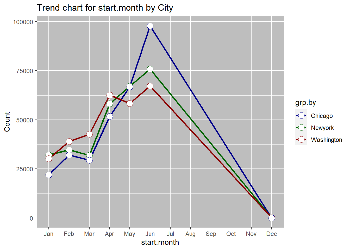
## $`Most Common Grouped`
## City start.month Grouped_ Count
## 1: Chicago Jun 97926
## 2: Newyork Jun 75895
## 3: Washington Jun 67239Get.Most.Common(dt$start.DOW, dt$City)## $`Most Common Overall`
## start.DOW Overall_ Count
## 1: Wed 140682
##
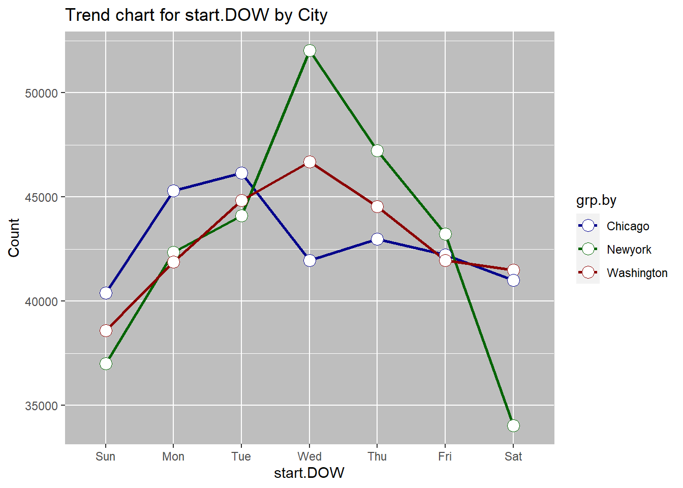
## $`Most Common Grouped`
## City start.DOW Grouped_ Count
## 1: Chicago Tue 46156
## 2: Newyork Wed 52040
## 3: Washington Wed 46684Get.Most.Common(dt$start.hourofday,dt$City)## $`Most Common Overall`
## start.hourofday Overall_ Count
## 1: 01 72670
##
## $`Most Common Grouped`
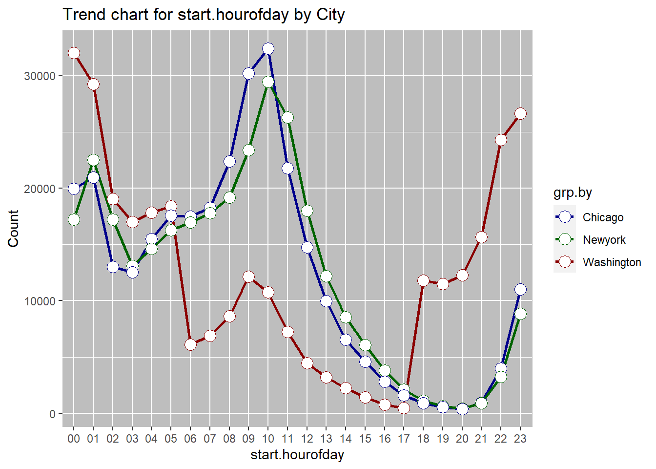
## City start.hourofday Grouped_ Count
## 1: Chicago 10 32415
## 2: Newyork 10 29468
## 3: Washington 00 32003- Freq.Categorical - creates frequency tables for categorical variable input combined for the three cities (overall) as well as broken down per city (grouped). The frequency table supplements the data visualizations created using ggplot2, if viewers need to take a look at exact numbers for a certain metric.
#function to calculate frequency tables and plots by metric
#1-deparse will get text out of user input - for creating dynamic plot labels
#2-Overall frequency followed by bygrp(by city) frequency table using data.table functions
#3 - c.palette specifies color palette for the bygrp(by city) plots.
#4-  create a list of ggplot items that are common to all plots.
#5 -Conditional (if else) to order by monthor by day - do this forboth overall and bygrp(by city)plots.
freq.categorical <- function(metric, grp.by){

      txt_usr_input1<- sub('...','',deparse((substitute(metric)))) #1
      txt_usr_input2<- sub('...','',deparse((substitute(grp.by))))
      temp.overall<- dt[, .N, by=.(metric)]#summarizing data
      overall <- temp.overall[order(-N)]                #2
      temp.bygrp <- dt[, .N, by=.(grp.by, metric)]
      bygrp <- temp.bygrp[order(dt, -N)] #2
      c.palette <- c("darkblue", "darkgreen", "darkred")
      #4 (for overall)
      p<- list(
          geom_bar(stat = "identity", fill = "darkblue"),
          ggtitle(paste0('Histogram for ', txt_usr_input1)),
          scale_y_continuous(labels = function(x) format(x, scientific = FALSE)),
          th1,labs(x = paste0(txt_usr_input1), y = 'Count')
      )
      #4 (for bygrp)
      p2 <- list(geom_line(size = 1) ,
                scale_y_continuous(labels = function(x) format(x, scientific = FALSE)),
                geom_point( size=4, shape=21,fill="white"),
                scale_color_manual(values = c.palette), th1,
                ggtitle(paste0('Trend chart for ', txt_usr_input1, ' by ', txt_usr_input2)),
                labs(x = paste0(txt_usr_input1), y = 'Count')
        )
      # 5 conditional
      #if DOW (string) in the argument, then factor the metric column with levels as ordered days of week with Sunday being first day
      if(str_detect(txt_usr_input1, "DOW")) {
          overall$metric <- factor(overall$metric,
                                  levels =c("Sun", "Mon", "Tue", "Wed", "Thu", "Fri", "Sat"))
          overall<- overall[order(overall$metric)]
          bygrp$metric <- factor(bygrp$metric,
                                  levels =c("Sun", "Mon", "Tue", "Wed", "Thu", "Fri", "Sat"))
          bygrp<- bygrp[order(bygrp$metric)]
          pltx <- ggplot(data=overall, aes_string(x=names(overall)[1], y = names(overall)[2])) + p
          plt2x<-ggplot(data=bygrp, aes_string(x=names(bygrp)[2], y=names(bygrp)[3], group = names(bygrp)[1], colour = names(bygrp)[1])) +p2
      print(pltx)
      print(plt2x)
      #elseif month(string) in the argument, then use the month.abb function to order month JAn - DEc
      }else if(str_detect(txt_usr_input1, "month")){
          pltx <-ggplot(data=overall, aes_string(x=names(overall)[1], y = names(overall)[2])) +
                 scale_x_discrete(limits = month.abb) + p
          plt2x<-ggplot(data=bygrp, aes_string(x=names(bygrp)[2], y=names(bygrp)[3], group = names(bygrp)[1], colour = names(bygrp)[1])) +
                 scale_x_discrete(limits = month.abb) + p2
      print(pltx)
      print(plt2x)
      # else plot and print
      }else{
          pltx <- ggplot(data=overall, aes_string(x=names(overall)[1], y = names(overall)[2])) + p
          plt2x<-ggplot(data=bygrp, aes_string(x=names(bygrp)[2], y=names(bygrp)[3], group = names(bygrp)[1], colour = names(bygrp)[1])) +p2
      print(pltx)
      print(plt2x)
      }

      result <- list("Overall"=overall, "Grouped"= bygrp) #combining summary result

return(result)

}

freq.categorical(dt$start.month, dt$City)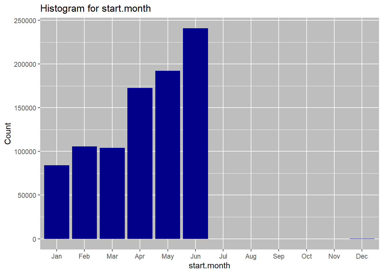
## $Overall
##    metric      N
## 1:    Jun 241060
## 2:    May 192159
## 3:    Apr 172609
## 4:    Feb 105773
## 5:    Mar 104074
## 6:    Jan  84186
## 7:    Dec    139
##
## $Grouped
##         grp.by metric     N
##  1:    Chicago    Jun 97926
##  2:    Newyork    Jun 75895
##  3: Washington    Jun 67239
##  4:    Newyork    May 67051
##  5:    Chicago    May 66816
##  6: Washington    Apr 62651
##  7: Washington    May 58292
##  8:    Newyork    Apr 58247
##  9:    Chicago    Apr 51711
## 10: Washington    Mar 42619
## 11: Washington    Feb 38975
## 12:    Newyork    Feb 34751
## 13:    Chicago    Feb 32047
## 14:    Newyork    Jan 32012
## 15:    Newyork    Mar 31983
## 16: Washington    Jan 30172
## 17:    Chicago    Mar 29472
## 18:    Chicago    Jan 22002
## 19:    Newyork    Dec    61
## 20: Washington    Dec    52
## 21:    Chicago    Dec    26
##         grp.by metric     N
freq.categorical(dt$start.DOW, dt$City)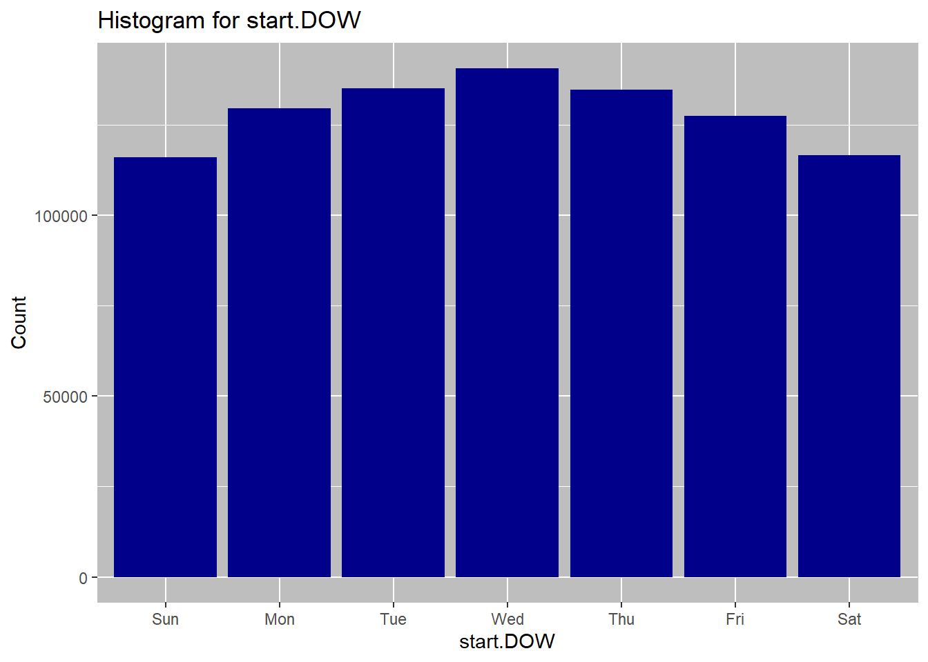
## $Overall
##    metric      N
## 1:    Sun 115985
## 2:    Mon 129529
## 3:    Tue 135083
## 4:    Wed 140682
## 5:    Thu 134752
## 6:    Fri 127429
## 7:    Sat 116540
##
## $Grouped
##         grp.by metric     N
##  1:    Chicago    Sun 40390
##  2: Washington    Sun 38582
##  3:    Newyork    Sun 37013
##  4:    Chicago    Mon 45291
##  5:    Newyork    Mon 42348
##  6: Washington    Mon 41890
##  7:    Chicago    Tue 46156
##  8: Washington    Tue 44833
##  9:    Newyork    Tue 44094
## 10:    Newyork    Wed 52040
## 11: Washington    Wed 46684
## 12:    Chicago    Wed 41958
## 13:    Newyork    Thu 47234
## 14: Washington    Thu 44545
## 15:    Chicago    Thu 42973
## 16:    Newyork    Fri 43230
## 17:    Chicago    Fri 42236
## 18: Washington    Fri 41963
## 19: Washington    Sat 41503
## 20:    Chicago    Sat 40996
## 21:    Newyork    Sat 34041
##         grp.by metric     N
freq.categorical(dt$start.hourofday, dt$City)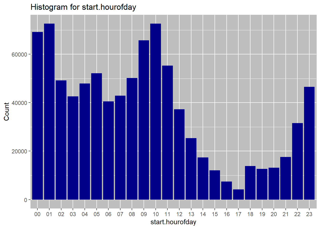
## $Overall
##     metric     N
##  1:     01 72670
##  2:     10 72636
##  3:     00 69154
##  4:     09 65736
##  5:     11 55292
##  6:     05 52167
##  7:     08 50178
##  8:     02 49233
##  9:     04 47922
## 10:     23 46492
## 11:     07 42907
## 12:     03 42633
## 13:     06 40576
## 14:     12 37254
## 15:     22 31537
## 16:     13 25362
## 17:     21 17540
## 18:     14 17355
## 19:     18 13830
## 20:     20 13141
## 21:     19 12697
## 22:     15 12085
## 23:     16  7398
## 24:     17  4205
##     metric     N
##
## $Grouped
##         grp.by metric     N
##  1:    Chicago     10 32415
##  2: Washington     00 32003
##  3:    Chicago     09 30183
##  4:    Newyork     10 29468
##  5: Washington     01 29228
##  6: Washington     23 26643
##  7:    Newyork     11 26273
##  8: Washington     22 24293
##  9:    Newyork     09 23395
## 10:    Newyork     01 22512
## 11:    Chicago     08 22368
## 12:    Chicago     11 21765
## 13:    Chicago     01 20930
## 14:    Chicago     00 19933
## 15:    Newyork     08 19164
## 16: Washington     02 19024
## 17: Washington     05 18372
## 18:    Chicago     07 18240
## 19:    Newyork     12 18006
## 20: Washington     04 17818
## 21:    Newyork     07 17770
## 22:    Chicago     05 17547
## 23:    Chicago     06 17496
## 24:    Newyork     00 17218
## 25:    Newyork     02 17207
## 26: Washington     03 16991
## 27:    Newyork     06 16969
## 28:    Newyork     05 16248
## 29: Washington     21 15655
## 30:    Chicago     04 15493
## 31:    Chicago     12 14764
## 32:    Newyork     04 14611
## 33:    Newyork     03 13097
## 34:    Chicago     02 13002
## 35:    Chicago     03 12545
## 36: Washington     20 12281
## 37:    Newyork     13 12201
## 38: Washington     09 12158
## 39: Washington     18 11783
## 40: Washington     19 11486
## 41:    Chicago     23 10997
## 42: Washington     10 10753
## 43:    Chicago     13  9970
## 44:    Newyork     23  8852
## 45: Washington     08  8646
## 46:    Newyork     14  8550
## 47: Washington     11  7254
## 48: Washington     07  6897
## 49:    Chicago     14  6551
## 50: Washington     06  6111
## 51:    Newyork     15  6067
## 52:    Chicago     15  4591
## 53: Washington     12  4484
## 54:    Chicago     22  4001
## 55:    Newyork     16  3813
## 56:    Newyork     22  3243
## 57: Washington     13  3191
## 58:    Chicago     16  2806
## 59: Washington     14  2254
## 60:    Newyork     17  2144
## 61:    Chicago     17  1592
## 62: Washington     15  1427
## 63:    Newyork     18  1144
## 64:    Chicago     21   952
## 65:    Newyork     21   933
## 66:    Chicago     18   903
## 67: Washington     16   779
## 68:    Newyork     19   667
## 69:    Chicago     19   544
## 70: Washington     17   469
## 71:    Newyork     20   448
## 72:    Chicago     20   412
##         grp.by metric     N
Step c) Results summary
June is the most common rental month overall, as well as for each of the cities. This may be driven by warm summer temperatures, tourists visitings due to school holidays etc. Wednesday is the most common day for start of the rentals overall. When broken down by the city, we see that wednesday is still the most comon rental start day for New York and washington, but for Chicgo the most common day of retnal start is Tuesday. weekday rentals may be higher due to workers commuting to work. Hourly data shows a bimodal distribution overall with 08:00am and 5:00pm being the most popular times for travel. This, again is likely due to the workers commuting to and from work at these hours. Trend by city shows the same dual peaks. The 5:00pm peak for washington is small, which may be due to overnight rentals.
amber.m.ahmed@utexas.edu
Copyright © , Amber Ahmed. All rights reserved.